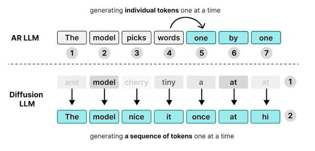
Diffusion models have revolutionized image generation, but applying them to language is trickier. Text is discrete, so you can’t just add Gaussian noise. This guide walks you through the key components noising, denoising, training, and sampling so you can build your own diffusion language model from scratch.

We’ll start with the core idea: instead of generating text left-to-right like GPT, a diffusion LM learns to reverse a gradual corruption process. By the end, you’ll understand the architecture choices, training objectives, and sampling tricks that make these models work and where they still struggle.

The Core Idea: Reversing Noise

Imagine you have a clean sentence: “The cat sat on the mat.” Now, over many steps, you progressively replace words with a placeholder like [MASK]. Eventually, you get a completely masked sequence: “[MASK] [MASK] [MASK] [MASK] [MASK] [MASK].” A diffusion language model learns to reverse this process—starting from pure noise and iteratively predicting the original tokens.

This is analogous to how image diffusion models work, but with a key difference: text is discrete. You can’t add continuous Gaussian noise to a token in a meaningful way. So researchers have developed several strategies to adapt diffusion to language.

Step 1: Choose Your Noising Process

The forward process corrupts a clean sequence over a fixed number of timesteps (e.g., T=1000). The choice of corruption determines the training objective and the model’s capabilities. Here are the most common approaches:

• Masking-based: At each timestep, randomly replace a fraction of tokens with a special [MASK] token. The fraction increases with timestep, so later steps are more corrupted. This is simple and effective, as seen in models like MDLM and BERT-style denoising.
• Multinomial diffusion: Instead of masking, you add noise over the categorical distribution of each token. Each token’s distribution is gradually pushed toward uniform—essentially, you’re replacing tokens with random ones with increasing probability.
• Continuous diffusion on embeddings: You embed tokens into a continuous vector space, then add Gaussian noise to the embeddings. This allows you to use standard continuous diffusion machinery, but you need a rounding step to convert denoised embeddings back to tokens.

For a first implementation, masking is the easiest to get right. It’s intuitive, and the training objective is straightforward cross-entropy on the masked positions.

Step 2: Design the Denoising Network

The reverse process is handled by a neural network that takes a corrupted sequence and predicts the original tokens. A transformer encoder is the natural choice because it can attend to all positions bidirectionally—a key advantage over autoregressive models.

You’ll feed in the corrupted token sequence, along with the timestep (as an embedding), and output probabilities for each token over the vocabulary. The architecture is similar to BERT, but you’ll add a timestep conditioning mechanism, like adaptive layer norm or additive embeddings.

The loss is typically cross-entropy between the predicted distribution and the original token at each masked position. In practice, you only compute the loss on positions that were corrupted, which forces the model to learn to reconstruct from context.

Step 3: Train the Model

During training, you sample a clean sequence from your dataset, randomly sample a timestep, and corrupt the sequence according to your noising process. Then you feed the corrupted sequence to the model and compute the loss.

A key trick is to use a mask schedule that determines how many tokens to mask at each timestep. For example, you might mask 50% of tokens at t=500, and 90% at t=900. The schedule can be uniform, linear, or cosine—choice affects training stability and final quality.

In practice, you’ll train for many steps on a large corpus. One challenge is that diffusion LMs are data-hungry and can be unstable to train. You may need to experiment with learning rates, gradient clipping, and the noise schedule.

Step 4: Sample by Denoising

To generate text, you start from a fully masked sequence (or a sequence of random tokens, depending on your noising process). Then, you iteratively apply the model: at each step, predict the original tokens, but only replace the most confident predictions (or use a schedule to gradually unmask).

For masking-based models, you typically use a strategy like confidence-based decoding: at each step, the model outputs probabilities for all masked positions. You unmask the top-k most confident tokens, then re-mask the remaining ones according to the schedule, and repeat. This is similar to how the MaskGIT model works for images, but for text.

Step 5: Handle Variable-Length Generation

One limitation of many diffusion LMs is that they work on fixed-length sequences. For text, you often need to generate variable-length outputs. A common trick is to use a start-of-sequence token and a special end-of-sequence token, but it’s tricky because the model doesn’t generate left-to-right.

One solution is to generate a fixed-length sequence that includes padding tokens, then post-process to trim. Another is to train with a length predictor or use a separate mechanism to decide when to stop.

Putting It All Together: A Minimal Example

Here’s a high-level pseudocode for training a masked diffusion LM:

python
for each batch of texts:
# 1. Sample a random timestep for each sequence
t = random.randint(0, T-1)
# 2. Corrupt the sequence according to the schedule
corrupted, mask = corrupt(text, t)
# 3. Feed corrupted sequence and timestep to the model
logits = model(corrupted, t)
# 4. Compute loss only on masked positions
loss = cross_entropy(logits, original_text, mask)
# 5. Backprop and update
loss.backward()
optimizer.step()

Sampling:

“`python

Start with a fully masked sequence

seq = [MASK] * max_length
for t in reversed(range(T)):
logits = model(seq, t)
probs = softmax(logits)
# Unmask the most confident tokens
confident = top_k(probs, k=int(schedule[t] * max_length))
seq[confident.indices] = confident.tokens

Return seq

“`

Challenges and Open Questions

Diffusion LMs are not yet competitive with autoregressive models on long-form generation quality. They often produce less coherent text and require many steps to generate, which can be slow. However, they excel in controllable tasks like infilling, where you have context on both sides.

Researchers are actively working on improving sampling efficiency (fewer steps), scaling laws, and hybrid approaches that combine autoregressive and diffusion elements. Some promising directions include using discrete diffusion with continuous-time schedules and flow matching techniques.

If you’re building one, expect to iterate on the noise schedule, architecture, and training tricks. But the field is moving fast, and diffusion LMs might soon become a practical alternative for certain applications.

Building a diffusion language model is a challenging but rewarding endeavor. By understanding the core components—noising, denoising, training, and sampling—you can implement your own and contribute to an open research frontier. While they may not yet match GPT-level quality, diffusion LMs offer unique advantages for controllability and parallel generation. Start with a simple masked diffusion model, and build from there.

Summary

• Diffusion LMs generate text by reversing a corruption process, unlike autoregressive models that generate left-to-right.
• Key components: a forward noising process (e.g., masking), a denoising network (transformer), and a training objective (cross-entropy on corrupted tokens).
• Sampling starts from pure noise and iteratively refines, often using confidence-based unmasking.
• Advantages: bidirectional context, parallel generation potential, and controllability.
• Challenges: training instability, variable-length generation, and quality gaps compared to autoregressive models.

FAQ

Q: What is the difference between autoregressive and diffusion language models?
A: Autoregressive models (like GPT) generate text one token at a time from left to right, each token conditioned on the previous ones. Diffusion LMs start from a noisy or masked sequence and iteratively refine it, using context from both sides.

Q: Why is text diffusion harder than image diffusion?
A: Images are continuous, so you can add Gaussian noise directly. Text is discrete—tokens are categorical—so you need to adapt the noising process, such as using masking or multinomial noise.

Q: What is a simple way to implement a diffusion LM?
A: Use masking as the noising process. Train a transformer encoder to predict masked tokens. For sampling, start with a fully masked sequence and iteratively unmask the most confident predictions.

Q: Do diffusion LMs perform as well as GPT models?
A: Not yet on standard benchmarks like long-form generation quality. However, they excel in controllable tasks like text infilling and offer potential for faster parallel generation.

Q: What are the main challenges in training diffusion LMs?
A: Training instability, choosing the right noise schedule, and handling variable-length output are common hurdles. You may need to experiment with hyperparameters and tricks like gradient clipping.