Tag: Performance

  • How to Build a 0ms Autocomplete for 240 Million Domain Names

    How to Build a 0ms Autocomplete for 240 Million Domain Names

    Imagine typing a domain name into a search box and seeing suggestions appear before your finger lifts off the key. For a dataset of 240 million domain names, that’s a massive technical challenge. A naive approach would scan every entry for each keystroke impossible at this scale. Yet some engineers claim to achieve P99 latency of 0 milliseconds (with an asterisk). How is that possible?

    This article breaks down the engineering behind such a feat, explaining the data structures, caching strategies, and trade-offs. We’ll explore what the asterisk means, why 0ms is both a real achievement and a clever marketing move, and whether you need such speed for your own autocomplete system.

    The Scale of the Problem

    240 million domain names is not just a big number—it’s about 70% of all registered domains across every TLD. To put it in perspective, imagine a phonebook with 240 million entries. If you wanted to find all names starting with “ab”, you’d have to scan every single page. That would take seconds, not milliseconds.

    For autocomplete, you need results in under 100ms for a human to perceive it as instant. But the challenge is worse: each keystroke changes the prefix, so you need to handle new queries in real time. A naive approach would be hopeless.

    The Classic Solutions and Their Limits

    Most autocomplete systems use one of these approaches:

    • Trie (prefix tree): A tree where each node represents a character. Traversing from root to a node gives a prefix. This is memory-hungry at scale—each node holds pointers to children, easily ballooning to tens of gigabytes.
    • Inverted index: A map from prefixes to lists of matching entries. Building this for all possible prefixes is expensive but makes lookup fast.
    • Finite State Transducers (FSTs): A compact automaton that encodes a set of strings efficiently. Lucene uses FSTs for its suggest feature, but even FSTs require traversing nodes, which takes microseconds.

    At 240 million entries, even a well-optimized trie traversal might take 1-10 milliseconds. To get to 0ms, you need a fundamentally different approach.

    The 0ms Trick: Precomputation and Caching

    The only way to achieve true 0ms server-side processing is to avoid computation altogether. The solution: precompute the results for every possible prefix (or a large subset) and store them in a hash map. Then, a lookup is O(1)—just a hash table read.

    For domain names, the prefixes you need to support are typically 1-3 characters long. There are 26^3 = 17,576 possible 3-letter prefixes. For each prefix, you precompute the top 10 most popular domain names starting with that prefix. Store these in a JSON file or a key-value store like Redis.

    When a user types “ab”, the server simply looks up the key “ab” and returns the precomputed list. No traversal, no ranking logic—just a hash lookup. That’s why the server-side time can be 0ms.

    But wait—where does the asterisk come in? The 0ms measurement excludes network time. The actual request still travels from the user’s browser to your server and back. That network round-trip might take 20-50ms. So the user doesn’t experience true 0ms, but the server processing is effectively instantaneous.

    The Memory Trade-Off

    Precomputing all prefixes is memory-intensive. For each of the 17,576 prefixes, you store a list of up to 10 domain names. If each domain name averages 15 characters, that’s about 150 characters per prefix. Multiply by 17,576, and you get roughly 2.6 million characters—about 2.6 MB of raw text. That’s surprisingly small! Even with overhead for data structures, you’re looking at maybe 10 MB.

    But what if you want to support longer prefixes, like “abou”? The number of possible 4-letter prefixes is 26^4 = 456,976. That’s still manageable—about 68 MB of raw text. For 5-letter prefixes, you’d have 11.8 million possibilities, which balloons to 1.7 GB. So you need to decide where to draw the line.

    Most autocomplete systems only need to handle prefixes up to 3 or 4 characters because users typically type a few letters before seeing results. For longer queries, you can fall back to a trie or a sorted array with binary search, which is still fast enough.

    The Cold Start Problem

    Precomputing results works great once the data is loaded into memory. But what happens on the first request after deployment? If you’re loading a 10 MB JSON file into a hash map, that might take a few hundred milliseconds. But that’s a one-time cost. After that, all lookups are fast.

    However, if you’re precomputing on the fly, you’d have a problem. The solution is to precompute offline, during deployment, and load the precomputed data into memory. This is a common pattern in high-performance systems.

    The Benchmark Caveat

    When the author writes “P99 0 ms*”, the asterisk typically points to a footnote: “Measured server-side, excluding network time.” This is a fair caveat because the user’s perceived latency includes network. But it’s also a bit of a marketing trick—0ms sounds amazing, but it’s not the full story.

    Moreover, P99 of 0ms means that 99% of requests were processed in under 1 millisecond (if the timer resolution is 1ms). That’s still incredibly fast, but it’s not literally zero. The point is that the server processing is so fast that it’s below the measurement threshold.

    Is 0ms Necessary?

    From a user experience perspective, 0ms is overkill. Human perception of instant is around 100ms. If your autocomplete responds in 50ms, users won’t notice any delay. The pursuit of 0ms is more about engineering bragging rights than practical need.

    However, there are scenarios where every millisecond counts, such as high-frequency trading interfaces or real-time collaborative tools. But for a domain name search, 100ms is perfectly fine.

    How to Implement This Yourself

    If you want to build a similar system, here’s a step-by-step approach:

    1. Collect your dataset: For domain names, you can get a list from public sources like Verisign’s COM/NET zone files or use a service like DomainIQ.
    2. Build a prefix map: For each prefix from 1 to 3 characters (or more if you wish), compute the top N suggestions. You can do this by sorting all domains and then extracting prefixes.
    3. Store the map: Save it as a JSON file or in a key-value store. If you’re using a CDN, you can serve static JSON files for each prefix, letting the CDN handle caching.
    4. Serve requests: When a user types a prefix, look up the key and return the list. If the prefix is longer than your precomputed limit, fall back to a secondary index (like a trie).
    5. Measure: Use high-resolution timers to measure server-side latency. You’ll likely see P99 of 0-1ms.

    The Trade-Offs and Limitations

    This approach sacrifices freshness. If you add new domains, you need to rebuild the precomputed map. For a domain name registrar, that might be acceptable if you update daily. But for a dynamic dataset, you’d need a more complex solution.

    Also, precomputing only top-N results means you might miss less popular matches. If a user types a rare prefix, you might not have any suggestions. But for autocomplete, you typically want popular results anyway.

    Finally, the memory footprint grows exponentially with prefix length. You need to choose a cutoff that balances coverage and memory.

    Conclusion

    Achieving P99 0ms autocomplete for 240 million domain names is possible through aggressive precomputation and caching. The asterisk reminds us that network time is excluded, but the server processing is genuinely instantaneous. While 0ms might be overkill for most applications, the techniques used—precomputation, hash maps, and CDN caching—are valuable for any high-performance autocomplete system. By understanding the trade-offs, you can decide how far to go in optimizing your own search features.

    The 0ms autocomplete is a testament to clever engineering—precomputing results for every possible prefix turns a computation problem into a simple lookup. While the asterisk hides the network latency, the server-side speed is real. For most builders, a 50ms response is plenty, but the principles of precomputation and caching can scale down to any dataset. If you’re looking to improve your autocomplete, consider whether you need 0ms or just fast enough.

    Summary

    • 240 million domain names is a massive dataset that rules out naive autocomplete.
    • The 0ms trick is to precompute results for every prefix and use a hash map for O(1) lookups.
    • The asterisk means the measurement excludes network time; server processing is truly near-zero.
    • Memory trade-offs: precomputing all 1-3 letter prefixes costs only ~10 MB, but longer prefixes balloon exponentially.
    • For most users, 50ms is imperceptible, so 0ms is a nice-to-have, not a necessity.

    FAQ

    Q: How can server processing be 0ms?
    A: By precomputing the results for every possible prefix and storing them in a hash map. Lookup is a simple hash read, which takes nanoseconds.

    Q: What does the asterisk () mean in ‘P99 0 ms‘?
    A: It usually means the measurement excludes network time. The server processing is 0ms, but the user still experiences network latency of 20-50ms.

    Q: Is 0ms necessary for a good user experience?
    A: No. Human perception of ‘instant’ is around 100ms. A 50ms response is indistinguishable from 0ms for most users.

    Q: What are the memory requirements?
    A: For all 1-3 letter prefixes (17,576 prefixes) with top 10 results each, you need about 10 MB. For 4-letter prefixes, it grows to ~70 MB.

    Q: How do I handle updates to the dataset?
    A: You need to rebuild the precomputed map whenever the dataset changes. This is fine for static data but less practical for highly dynamic data.


  • The Science Behind Why We Talk to Ourselves (And When It’s a Problem)

    The Science Behind Why We Talk to Ourselves (And When It’s a Problem)

    You’re not crazy if you talk to yourself. In fact, you’re engaging in a normal, often beneficial cognitive process that scientists have studied for decades. From helping children learn to guiding athletes to victory, self-talk is a powerful tool. But when does this internal dialogue cross the line into a clinical concern? Let’s explore the science behind self-talk, its benefits, and the warning signs to watch for.

    What Is Self-Talk?

    Self-talk is the dialogue you have with yourself, whether it’s out loud, whispered, or purely in your head. It’s a common phenomenon; studies estimate that people spend 25% to 50% of their waking hours engaged in some form of internal dialogue. This chatter can be instructional (“Turn left at the next street”), motivational (“You’ve got this!”), or evaluative (“That was a stupid mistake”).

    Self-talk emerges early in life. Around age 2–3, children start talking to themselves out loud, a behavior psychologists call “private speech.” This is completely normal and serves a crucial developmental purpose. By age 5–7, most children internalize this speech, turning it into the silent inner voice we experience as adults. This transition is tied to language development and executive function—the mental skills that help us plan, focus, and multitask.

    The Brain’s Inner Voice

    When you talk to yourself, your brain lights up in specific ways. Neuroimaging studies using fMRI show that inner speech activates the left inferior frontal gyrus (known as Broca’s area) and the left superior temporal gyrus (Wernicke’s area)—the same regions responsible for producing and understanding external speech. Even silent self-talk produces subtle activation in the motor cortex, the part of the brain that controls movement. This suggests that “talking to yourself” is neurologically similar to actually speaking, just without the vocalization.

    This neural overlap explains why self-talk can be so effective. By engaging the same brain circuits used for real speech, self-talk harnesses the power of language to organize thoughts, regulate emotions, and guide behavior.

    The Benefits of Self-Talk

    Performance Enhancement

    Research by psychologist Antonis Hatzigeorgiadis and colleagues at the University of Thessaly has shown that instructional self-talk—phrases like “focus,” “step,” or “breathe”—can significantly improve performance in tasks requiring fine motor skills, concentration, and sports performance. For example, tennis players who use instructional self-talk to remind themselves to watch the ball or bend their knees tend to hit more accurate shots. Similarly, students who tell themselves to “pay attention” during a difficult lecture often retain more information.

    Motivation and Emotional Regulation

    Self-talk also has motivational power. Interestingly, studies suggest that using second-person self-talk (“You can do this”) is more effective than first-person (“I can do this”) for regulating emotions and motivating behavior under stress. Why? Because talking to yourself as “you” creates psychological distance, allowing you to view the situation more objectively, as if advising a friend. This distancing effect can reduce anxiety and boost confidence, making it a valuable tool in high-pressure situations like job interviews or public speaking.

    Cognitive Development

    Lev Vygotsky, a Russian psychologist, proposed in the 1930s that private speech is a critical developmental tool. Children use it to guide their actions and solve problems, like when a toddler says “put the block here” while building a tower. Vygotsky argued that this external speech eventually becomes internalized as inner speech, which we use for self-regulation and planning. His theory has been widely supported by modern research, and contemporary cognitive science treats self-talk as a key component of self-control and problem-solving.

    When Self-Talk Becomes a Problem

    Despite its benefits, self-talk can sometimes signal or contribute to mental health issues. It’s important to note that talking to yourself out loud is not inherently pathological. The vast majority of self-talk is healthy and normal. However, there are two main scenarios where self-talk becomes a concern.

    Negative Rumination

    Maladaptive rumination is repetitive, negative, self-critical self-talk, such as “I’m worthless,” “I always fail,” or “Nobody likes me.” This type of self-talk is a hallmark of depression and anxiety disorders. It can trap you in a cycle of negativity, reinforcing low self-esteem and hopelessness. Cognitive-behavioral therapy (CBT) often targets this kind of self-talk by helping individuals identify and challenge these automatic negative thoughts, replacing them with more balanced, realistic ones.

    Auditory Hallucinations vs. Self-Talk

    A key distinction is between self-talk and auditory hallucinations. Hallucinations involve hearing voices that seem external and are not your own. They are associated with conditions like schizophrenia, bipolar disorder with psychotic features, and severe depression. In contrast, self-talk is your own voice, whether internal or external, and you know it’s you. If you hear voices that feel alien or out of your control, it’s important to seek professional help.

    The Fine Line Between Healthy and Unhealthy

    So, how do you know if your self-talk is a problem? Here are some red flags:

    • Frequency and intensity: If self-talk becomes intrusive, constant, or hard to control, it may be a sign of anxiety or obsessive thinking.
    • Content: If your self-talk is predominantly negative, self-critical, or worrisome, it could be contributing to depression or anxiety.
    • Functional impairment: If self-talk interferes with your daily functioning—for example, you can’t concentrate or complete tasks because of excessive internal dialogue—it’s worth addressing.
    • Dissociation from reality: If you start believing your self-talk is an external voice or that others can hear your thoughts, this could indicate a more serious condition.

    In these cases, consulting a mental health professional can help you develop strategies to manage your self-talk and improve your well-being.

    Conclusion

    Talking to yourself is a natural and beneficial part of being human. It helps you learn, perform, and regulate your emotions. By understanding the science behind self-talk, you can harness its power to improve your life. But it’s also crucial to recognize when self-talk becomes negative or pathological, and to seek help when needed. So next time you catch yourself muttering under your breath, remember: you’re in good company.

    Self-talk is a powerful cognitive tool that serves us from childhood through adulthood. Whether you’re rehearsing a presentation, giving yourself a pep talk, or working through a problem, your inner voice is there to help. But keep an ear out for the warning signs—persistent negativity, loss of control, or a shift in reality—because those indicate it’s time to seek support. Talk to yourself, but make sure it’s a conversation that empowers you.

    Summary

    • Self-talk is a normal and common behavior, with people spending 25-50% of waking hours in internal dialogue.
    • It begins in childhood as external private speech and becomes internalized by age 5-7.
    • The same brain areas used for external speech are active during inner speech, making self-talk a powerful cognitive tool.
    • Instructional self-talk improves focus and performance; second-person self-talk enhances motivation and emotional regulation.
    • Self-talk becomes a concern when it’s persistently negative (rumination) or when it manifests as auditory hallucinations, indicating a need for professional help.

    FAQ

    Q: Is talking to yourself a sign of mental illness?
    A: No, not by itself. Talking to yourself is a normal and common behavior. It only becomes a concern when it’s accompanied by other symptoms, like persistent negativity or auditory hallucinations.

    Q: What’s the difference between self-talk and auditory hallucinations?
    A: Self-talk is your own voice, and you know it’s you. Auditory hallucinations involve hearing voices that seem external and not your own, and they’re associated with conditions like schizophrenia. If you experience hallucinations, seek professional help.

    Q: How can I use self-talk to improve my performance?
    A: Use instructional self-talk (e.g., “focus,” “breathe”) during tasks requiring concentration. For motivation under stress, try second-person self-talk (“You can do this”) to create psychological distance.

    Q: When should I be concerned about my self-talk?
    A: Be concerned if your self-talk is predominantly negative, intrusive, or hard to control, or if it interferes with daily functioning. These signs may indicate depression, anxiety, or another condition that could benefit from professional support.

    Q: Can children’s self-talk be encouraged?
    A: Yes. Vygotsky’s research shows that private speech helps children solve problems and regulate behavior. Encouraging self-talk in educational settings can support learning and development.

  • When ‘Clean’ Code Becomes a Performance Nightmare

    When ‘Clean’ Code Becomes a Performance Nightmare

    In the world of software development, ‘clean code’ is often treated as the holy grail. We’re taught to write small, focused functions, use interfaces, and avoid ‘premature optimization.’ But what if these well-intentioned practices are secretly sabotaging your application’s speed? In 2023, game developer Casey Muratori sparked a heated debate with his essay ‘Clean Code, Horrible Performance,’ showing how ‘clean’ abstractions can make code 2 to 10 times slower—or worse—even with modern optimizing compilers. This isn’t just a niche concern for game developers; it’s a wake-up call for anyone building performance-sensitive software, from web services to mobile apps.

    In this article, we’ll break down Muratori’s core argument, explore why ‘clean’ code can be so costly, and offer a balanced perspective on when to prioritize performance over purity. You’ll learn why a straightforward, ‘ugly’ implementation often beats a beautifully abstracted one, and how to make informed trade-offs in your own projects.

    The Tale of Two Codebases

    Imagine you’re building a simple game where you have a bunch of entities—say, spaceships—that need to update their positions each frame. You have two ways to write this.

    The ‘Clean’ Way:
    – Define an Entity interface with a virtual update() method.
    – Create separate classes like Spaceship, Asteroid, etc., each implementing update().
    – Use dependency injection to pass in a PhysicsEngine to each entity.
    – Wrap all data in getters and setters to ‘protect’ it.

    The ‘Ugly’ Way:
    – Use a simple struct with plain public fields.
    – Write a single function that loops over an array of these structs and updates them directly.

    Muratori’s article demonstrates that the ‘clean’ version can be 2 to 10 times slower than the ‘ugly’ one. Why? Because the ‘clean’ abstractions—virtual functions, interfaces, getters/setters—create layers of indirection that the compiler can’t see through. It can’t inline the virtual call, it can’t vectorize the loop because it doesn’t know which concrete type it’s dealing with, and it can’t eliminate dead code because the interface hides what’s actually happening.

    The Compiler’s Dilemma

    To understand why ‘clean’ code is slow, you need to understand how modern compilers optimize. Compilers like GCC, Clang, and MSVC are incredibly good at optimizing simple, flat code. They can inline small functions, vectorize loops to use SIMD instructions, and eliminate unused code—all in milliseconds. But they’re also incredibly fragile. The moment you introduce a virtual function, a function pointer, or an opaque interface, the compiler’s ability to optimize plummets.

    Here’s a concrete analogy: think of the compiler as a chef who can prepare a meal much faster if they know exactly what ingredients they have. If you hand them a sealed box (an interface) and say ‘cook whatever’s inside,’ they have to open it, inspect it, and then decide—that takes time. But if you hand them a clear container with labeled ingredients (a plain struct), they can start cooking immediately, even combining steps.

    In code, a virtual function call means the compiler doesn’t know which function will be called at runtime. It has to look up the function pointer in a vtable, which prevents inlining. Inlining is crucial for performance because it eliminates the overhead of a function call and allows further optimizations across function boundaries. Without inlining, every call has overhead, and the compiler can’t optimize the code inside the function in the context of the caller.

    Similarly, getters and setters—even if they’re inline—can prevent the compiler from seeing the actual data layout. If you have a class with private fields and only access them via getters, the compiler might not be able to reorder or combine operations as effectively as it could with direct field access.

    The Real-World Impact

    You might be thinking, ‘So what? My app isn’t a game. It’s a CRUD app that’s mostly waiting on database queries.’ That’s a fair point. For I/O-bound applications, CPU performance is rarely the bottleneck. But consider these scenarios:

    • Cloud Computing Costs: If your service is CPU-bound, a 10x performance hit means you need 10x more servers to handle the same load. That’s a direct financial cost. In 2023, with cloud costs rising, this is a serious concern.
    • Real-Time Systems: In game development, frame rate is a product feature. A slow update loop means dropped frames, which players notice immediately. Muratori’s example is from a game, but the same applies to VR, AR, and any real-time simulation.
    • Data Processing: If you’re processing large datasets—like in machine learning or analytics—a 2x slowdown can turn a 10-minute job into a 20-minute one. Multiply that by thousands of jobs, and you’ve got a significant efficiency loss.

    Even in web development, JavaScript engines like V8 are excellent at optimizing hot paths, but they too struggle with dynamic dispatch and heavy abstraction. So the principles apply beyond C++.

    The ‘Clean Code’ Defense

    Now, let’s play devil’s advocate. Defenders of clean code argue that performance isn’t everything. Maintainability, team velocity, and bug reduction often matter more. They point out that Muratori’s examples are cherry-picked—they’re CPU-bound loops where performance is critical, but most business applications are I/O-bound. They also cite Knuth’s famous quote: ‘Premature optimization is the root of all evil.’

    There’s truth to this. If you’re building a simple CRUD app, obsessing over micro-optimizations is a waste of time. But the counter-argument is that ‘clean’ code often isn’t just ‘not optimized’—it’s actively slow. And the problem is that once you’ve built a system with layers of abstraction, it’s very hard to optimize later without a major refactor. So the choice isn’t ‘optimize now’ vs. ‘optimize later’; it’s ‘write simple, fast code now’ vs. ‘write abstract, slow code and hope you can fix it later.’

    The Middle Ground: Know Your Hot Paths

    The real lesson from Muratori’s article isn’t ‘clean code is bad’ or ‘performance is everything.’ It’s that you need to know your performance budget. Not every line of code needs to be optimized, but the hot paths—the code that runs most frequently—deserve special attention.

    A practical approach is to:

    1. Measure first. Use a profiler to find where your code spends most of its time. Don’t guess.
    2. Write simple, flat code for hot paths. Avoid virtual functions, interfaces, and excessive abstraction in loops that run millions of times.
    3. Use ‘clean’ practices where they matter. Naming, formatting, and small functions are great for readability and don’t hurt performance. The problem is unnecessary abstraction, not cleanliness per se.
    4. Consider data-oriented design. Instead of thinking in terms of objects, think in terms of data and how it’s laid out in memory. This often leads to better cache locality and vectorization.

    A Concrete Example

    Let’s look at a simplified version of Muratori’s example to make it concrete. Suppose you have a Particle class with a virtual update() method:

    “`cpp
    class Particle {
    public:
    virtual void update(float dt) = 0;
    };

    class MovingParticle : public Particle {
    public:
    void update(float dt) override {
    x += vx * dt;
    y += vy * dt;
    }
    private:
    float x, y, vx, vy;
    };
    “`

    Now, if you have a vector of Particle* and call update() on each, the compiler can’t inline the call because it doesn’t know the concrete type. It has to do a vtable lookup for each particle.

    In contrast, a data-oriented approach might look like:

    “`cpp
    struct Particle {
    float x, y, vx, vy;
    };

    void updateParticles(Particle* particles, int count, float dt) {
    for (int i = 0; i < count; ++i) {
    particles[i].x += particles[i].vx * dt;
    particles[i].y += particles[i].vy * dt;
    }
    }
    “`

    This version is trivially vectorizable—the compiler can use SIMD to process multiple particles at once. It’s also cache-friendly because the data is contiguous. The result is a massive speedup, often 2-10x or more.

    The Bigger Picture

    Muratori’s article is part of a larger movement toward performance-aware programming, championed by people like Mike Acton and the data-oriented design community. They argue that the way we teach software engineering—with a focus on OOP and abstraction—is fundamentally at odds with how modern CPUs work. CPUs are optimized for sequential, predictable access patterns, not for jumping through pointers.

    This doesn’t mean OOP is useless. It’s great for organizing large codebases and modeling complex domains. But it’s a tool, not a universal solution. For performance-critical code, you need to think about data layout, cache behavior, and compiler optimizations.

    In 2023, this debate is more relevant than ever. With the rise of AI code generation, ‘clean’ patterns are often auto-generated, potentially baking in performance issues. And with cloud costs soaring, performance is a financial issue, not just a technical one.

    So, what should you do? Start by measuring your code. Find your hot paths. And don’t be afraid to write ‘ugly’ code if it’s fast. Your users—and your wallet—will thank you.

    The ‘clean code vs. performance’ debate isn’t about choosing one over the other. It’s about being intentional. Clean code is valuable for maintainability, but it shouldn’t come at the cost of 10x performance losses in critical sections. By understanding how compilers work and where your hot paths are, you can make informed trade-offs. Write clean code where it matters, and write fast, simple code where it counts. Measure, optimize, and repeat.

    Summary

    • ‘Clean’ code practices like virtual functions, interfaces, and getters/setters can make code 2-10x slower by preventing compiler optimizations like inlining and vectorization.
    • Modern compilers excel at optimizing simple, flat code but fail with layers of indirection.
    • Performance matters not just for games but for cloud costs, real-time systems, and data processing.
    • The solution is to know your hot paths, measure performance, and use data-oriented design for critical loops.
    • The debate is not about rejecting clean code entirely but about avoiding unnecessary abstraction in performance-sensitive areas.

    FAQ

    Q: Does this mean I should never use interfaces or virtual functions?
    A: No. Interfaces and virtual functions are useful for extensibility and decoupling. The key is to avoid them in hot paths—code that runs frequently, like loops and update methods. Use them for high-level architecture, but keep the low-level performance-critical code simple and concrete.

    Q: Is this only a C++ problem?
    A: No. Any language with virtual dispatch or dynamic typing (Java, C#, Python, JavaScript) suffers similar issues. Even JIT-compiled languages like Java can struggle with megamorphic call sites. The principles apply broadly.

    Q: What is data-oriented design?
    A: Data-oriented design is an approach that focuses on how data is laid out in memory and accessed, rather than on objects and their relationships. It emphasizes contiguous arrays, cache locality, and batch processing, which often leads to better performance.

    Q: How do I know if my code is performance-critical?
    A: Use a profiler. Identify functions that consume a significant portion of CPU time or are called millions of times. These are your hot paths. Optimize those, and leave the rest as clean as you like.

    Q: Can’t I just optimize later?
    A: You can, but it’s often harder. Refactoring a heavily abstracted system to be fast can require significant rewrites. It’s better to write simple, fast code from the start for hot paths, and add abstraction only where it doesn’t hurt performance.

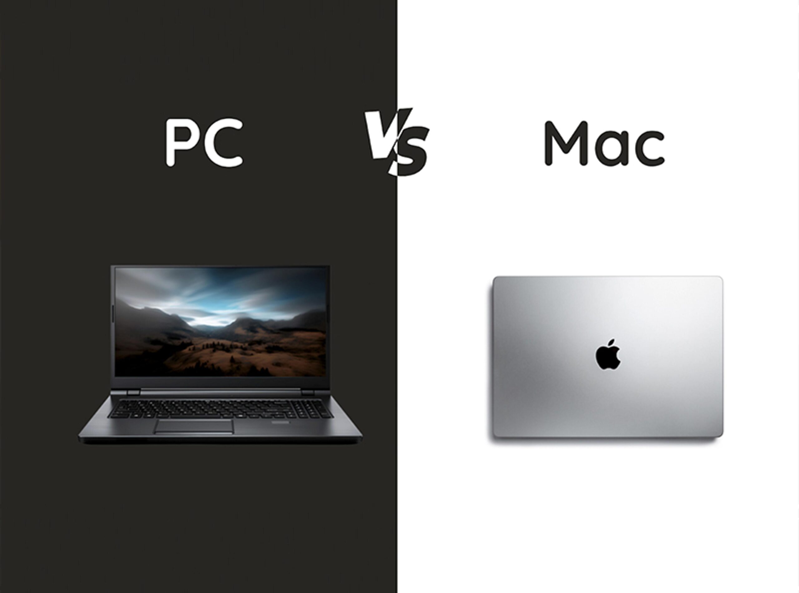
  • Mac vs PC for Video Editing: A Practical Guide for 2024

    Mac vs PC for Video Editing: A Practical Guide for 2024

    Choosing between a Mac and a PC for video editing is one of the most debated decisions in the creative world. With Apple’s shift to its own silicon and NVIDIA’s powerful GPUs, the landscape has changed dramatically. This guide breaks down the key differences—performance, software, price, and workflow—to help you make an informed choice based on your specific needs.

    Whether you’re a solo YouTuber, a professional colorist, or a student just starting out, the right platform can save you hours of render time and frustration. But there’s no one-size-fits-all answer. The best choice depends on the codecs you shoot, the software you use, and whether you value portability or upgradability.

    The Hardware Landscape: Apple Silicon vs. PC Components

    Since 2020, Macs have used Apple’s M-series chips (M1, M2, M3, and M4). These chips use a unified memory architecture, meaning the CPU and GPU share the same RAM. This design allows for fast data access and includes dedicated media engines that accelerate video encoding and decoding for formats like H.264, HEVC, and ProRes. In contrast, PCs are built from separate components: Intel or AMD processors, NVIDIA or AMD graphics cards, and system RAM. High-end editing PCs typically feature 32–64GB of RAM, 8–16 core CPUs, and GPUs with 8–24GB of VRAM.

    For video editing, the hardware matters because it directly impacts timeline smoothness, render times, and effects performance. Macs excel at tasks that leverage their media engines, especially ProRes workflows. PCs, on the other hand, shine when you need raw multi-core processing or GPU-accelerated effects, especially with NVIDIA’s CUDA technology.

    Software Support: What Runs Where?

    Most major editing software is available on both platforms. Adobe Premiere Pro, DaVinci Resolve, and After Effects have near-feature parity on Mac and PC. Avid Media Composer, the industry standard for film and TV, also runs on both. The big exception is Final Cut Pro, which is Mac-only. Final Cut Pro is a one-time purchase (around $299) and is known for its magnetic timeline and background rendering, making it a favorite for fast, efficient editing.

    DaVinci Resolve deserves special mention because its free version is remarkably capable on both platforms. The Studio version adds features like noise reduction and HDR grading. If you’re using Resolve, the choice between Mac and PC often comes down to GPU performance—NVIDIA GPUs on PCs are heavily optimized for Resolve, but Macs handle ProRes natively.

    Performance Benchmarks: Real-World Trends

    In 2023–2024, performance between Macs and PCs is closer than ever. For ProRes workflows, Macs (especially M3/M4 Pro and Max models) have a clear advantage due to hardware acceleration. If you shoot on an iPhone or use ProRes for delivery, a Mac will feel snappy. For raw formats like RED, BRAW, or ARRIRAW, high-end PCs with NVIDIA GPUs often match or beat Macs, especially for GPU-accelerated effects and rendering.

    Export times are often comparable in real-world tests. Macs tend to win on battery efficiency and thermal management in laptops, while PCs win on raw multi-core rendering in some workloads. For 8K editing and heavy color grading, both can handle it, but PCs scale better with multiple GPUs—Macs don’t support multi-GPU setups.

    Price and Upgradability: The Long-Term Cost

    Macs are generally more expensive upfront. A MacBook Pro 14 or 16-inch with an M3 Pro or Max chip starts around $1,999–$2,499. The Mac Studio with an M2 Ultra is over $3,999. And once you buy a Mac, you can’t upgrade the RAM or storage later—they’re soldered to the motherboard.

    PCs, on the other hand, range from $1,200 for an entry-level build to $5,000+ for a high-end workstation. You can upgrade RAM, storage, and GPU over time, extending the useful life of your machine by years. This makes PCs a better long-term investment if you’re willing to tinker. However, Macs hold their resale value better, so you can recoup some cost when you sell.

    The Mac-First Argument: Why Many Editors Choose Apple

    Final Cut Pro’s magnetic timeline is a game-changer for many editors—it automatically handles clip connections and trims, saving time. ProRes is the industry standard for delivery, and Macs handle it natively, so you’ll see smooth playback and fast exports. Battery life and portability are unmatched in the MacBook Pro, making it ideal for on-location editing. The machines are also silent, even under load, which is a real benefit in a quiet studio. macOS is stable and less prone to driver issues than Windows.

    The PC-First Argument: Why Power Users Prefer PCs

    Upgradability is the biggest advantage. You can add RAM, swap GPUs, and expand storage, which can extend the life of your system by 2–3 times. NVIDIA’s CUDA acceleration is heavily optimized in DaVinci Resolve, After Effects, and Blender, so if you use these tools, a PC with an RTX GPU will give you excellent performance. Cost per frame is often better on PCs—you get more raw performance for your dollar, especially for rendering. Windows also runs more software, including some plugins and 3D tools like Unreal Engine. And PCs are easier and cheaper to repair, with no need to visit an Apple Store.

    The Nuanced View: It Depends on Your Workflow

    Ultimately, the best choice depends on your specific situation. If you shoot ProRes, a Mac is a no-brainer. If you shoot BRAW or RED, a PC (or a high-end Mac) will give you better performance. If you use Premiere or Avid, either platform works. If you use Final Cut Pro, you must get a Mac. If you use DaVinci Resolve, a PC with an NVIDIA GPU is often the best value.

    Form factor also matters. If you need a laptop, the MacBook Pro is the best editing laptop on the market. If you want a desktop tower with maximum power, a PC is the way to go. And consider long-term cost: Macs cost more upfront but hold value, while PCs cost less but may need upgrades sooner.

    The Hybrid Approach: Using Both

    Many professionals use both platforms. A MacBook Pro for field editing and client meetings, and a PC workstation for heavy rendering and 3D work. This gives you the best of both worlds, though it requires managing two ecosystems. If you have the budget, this is the most flexible setup.

    There’s no definitive winner in the Mac vs PC debate—it all comes down to your workflow, budget, and preferences. Macs offer seamless ProRes support, portability, and a polished user experience. PCs offer upgradability, GPU flexibility, and often better value for raw performance. Consider what you shoot, what software you use, and whether you need a laptop or desktop. By weighing these factors, you’ll find the platform that lets you focus on your creative work, not your hardware.

    Summary

    • Macs excel at ProRes workflows and offer unmatched portability and battery life, especially in the MacBook Pro.
    • PCs offer upgradability and GPU flexibility, with NVIDIA CUDA acceleration boosting performance in Resolve and After Effects.
    • Software support is nearly identical except for Final Cut Pro, which is Mac-only.
    • Performance is comparable in most real-world tests, but PCs scale better with multi-GPU setups.
    • Price and long-term cost: Macs cost more upfront but hold value; PCs are cheaper to upgrade and repair.

    FAQ

    Q: Is a Mac or PC better for video editing?
    A: It depends on your workflow. Macs are better for ProRes and Final Cut Pro, while PCs are better for GPU-heavy tasks and upgradability.

    Q: Can I use Final Cut Pro on a PC?
    A: No, Final Cut Pro is only available on macOS.

    Q: Do I need a dedicated GPU for video editing?
    A: Yes, a dedicated GPU is essential for smooth playback and fast rendering, especially with effects and color grading.

    Q: Are Macs more expensive than PCs?
    A: Generally, yes, Macs have a higher upfront cost, but they hold resale value better. PCs can be cheaper to upgrade over time.

    Q: Which is better for DaVinci Resolve?
    A: Both work well, but PCs with NVIDIA GPUs often offer better performance due to CUDA acceleration. Macs handle ProRes natively, which is a plus if you use that codec.

  • Java’s Value Objects: A New Era for Performance and Simplicity

    Java’s Value Objects: A New Era for Performance and Simplicity


    Java has always been a language of objects. But every object comes with a hidden cost: a unique identity, a monitor for synchronization, and a memory overhead that can bloat your applications. For decades, developers have dreamed of a way to get the performance of primitives with the flexibility of objects. That dream is finally becoming a reality with JEP 401: Value Objects (Preview), which has just been merged into the OpenJDK master branch.

    This merge is a major milestone for Project Valhalla, an ambitious initiative to bring value types to Java. It promises to reshape how we write high-performance code, making Java more competitive with languages like C++ and Rust for data-intensive applications. But what exactly are value objects, and why should you care? In this article, we’ll break down the concept, explore the implications, and separate the hype from the reality.

    The Problem with Java’s Objects

    Imagine you’re building a 3D graphics engine. You need to store millions of points, each with x, y, and z coordinates. In Java, you’d likely create a class like this:

    java
    class Point {
    final double x;
    final double y;
    final double z;
    // constructor, getters, etc.
    }

    Then you’d store them in an array: Point[] points = new Point[1_000_000];

    But here’s the catch: each Point object is a full-fledged Java object. That means each one has an object header (typically 12-16 bytes) that stores metadata like the class pointer, identity hash code, and lock state. On top of that, the array stores references to these objects, not the objects themselves. So you have an array of 8-byte references, each pointing to a separate object in memory. This leads to:

    • Memory bloat: Each point takes up significantly more memory than just the three doubles (24 bytes) – often 40-50 bytes or more.
    • Poor cache locality: The objects are scattered across memory, so the CPU can’t efficiently load them into cache.
    • GC pressure: Millions of small objects put a heavy load on the garbage collector.

    This is why Java has a reputation for being memory-hungry compared to languages with structs or plain old data (POD) types.

    Enter Value Objects

    JEP 401 introduces a new kind of class: a value class. You declare it with the value modifier:

    java
    value class Point {
    final double x;
    final double y;
    final double z;
    // constructor, getters, etc.
    }

    Value classes have strict rules:

    • Final fields only: All fields must be final. This ensures immutability.
    • No identity: Instances have no unique identity. You can’t use == to compare them (only equals()), and you can’t synchronize on them.
    • No null: A value object can’t be null. Instead, it has a default value (like 0 for primitives).

    These rules allow the JVM to treat value objects like primitives. When you store them in an array, the JVM can flatten them – meaning the array stores the actual field values directly, without object headers or references. So Point[] becomes a contiguous block of memory with just the x, y, z values, just like a double[] but with three dimensions.

    This is a game-changer for performance. Memory usage drops dramatically, cache locality improves, and garbage collection pressure decreases because there are no individual objects to manage.

    How It Works Under the Hood

    The magic happens in the JVM’s object model. For value classes, the JVM can generate specialized code that:

    • Flattens fields: When a value object is stored in an array or as a field of another object, its fields are inlined directly, eliminating the object header and pointer indirection.
    • Uses stack allocation: Value objects can be allocated on the stack instead of the heap, further reducing overhead.
    • Optimizes method calls: Since value objects are immutable and have no identity, the JIT compiler can aggressively optimize calls to their methods, potentially inlining them.

    This is similar to how C++ structs work, but with Java’s safety guarantees (like null-safety and immutability).

    The Road to JEP 401

    This JEP is the culmination of over a decade of work on Project Valhalla. Earlier prototypes explored different syntaxes and semantics, but the community settled on a simplified approach: the value modifier on a class. The key is that value classes are a natural extension of records (introduced in Java 16). In fact, you can combine them:

    java
    value record Point(double x, double y, double z) {}

    This gives you the concise syntax of a record with the performance of a value type.

    What This Means for Developers

    Performance Gains

    The most obvious benefit is performance. For applications that deal with large collections of simple data – such as scientific computing, game development, or financial modeling – value objects can reduce memory usage by 50% or more and significantly speed up access times.

    API Design

    Value objects change how you design APIs. Since they have no identity, you can’t rely on == for comparisons. You must use equals(). Also, value objects can’t be null, so you need to handle default values explicitly. This might require a shift in thinking for some developers.

    Library Compatibility

    Libraries that rely on identity (e.g., using == for caching) will need to be updated. For example, HashMap uses hashCode() and equals(), which work fine with value objects, but some internal optimizations might not apply. The Java standard library will need to be audited to ensure it works efficiently with value types.

    The Preview Status

    JEP 401 is a preview feature. That means it’s not enabled by default. To use it, you must compile and run with --enable-preview. The API and semantics are subject to change based on developer feedback. This is a chance for the community to experiment and provide input before the feature is finalized.

    Potential Pitfalls

    • Misuse: Value classes are not a silver bullet. If you create a value class with many large fields (e.g., a byte[]), flattening might not help, and you could end up with worse performance due to copying.
    • Complexity: The JVM changes are complex, and there might be edge cases that cause unexpected behavior. The preview status means you should test thoroughly.
    • Ecosystem adoption: It will take time for libraries and frameworks to take advantage of value types. In the meantime, you might not see immediate benefits in your existing codebase.

    The Future

    JEP 401 is just the beginning. Future JEPs will likely build on this foundation, possibly adding more features like specialized generics (so you can have List<int> without boxing) and further optimizations. The ultimate goal is to make Java a first-class language for high-performance computing.

    Conclusion

    JEP 401 is a monumental step for Java. By introducing value objects, the language is finally addressing one of its biggest weaknesses: the overhead of object-oriented programming. While the feature is still in preview, it’s a clear signal that Java is evolving to meet the demands of modern computing. Whether you’re a performance enthusiast or a cautious developer, now is the time to start experimenting with value objects and see how they can transform your code.

    Value objects are not just a new language feature; they represent a fundamental shift in how Java handles data. By flattening objects into their fields, the JVM can achieve performance levels previously only possible with primitives or native code. As the feature matures and gains broader adoption, we can expect to see a new wave of Java applications that are faster, more memory-efficient, and more scalable. The merge of JEP 401 into OpenJDK master is a historic moment, and the future of Java looks brighter than ever.

    Summary

    • What: JEP 401 introduces value objects (value classes) to Java, allowing user-defined types with primitive-like performance.
    • Why: To reduce memory overhead and improve cache locality for large collections of simple data.
    • How: Value classes are immutable, have no identity, and can be flattened by the JVM into their fields.
    • Status: Preview feature, merged to OpenJDK master; requires --enable-preview to use.
    • Impact: Potential for significant performance gains in data-intensive applications, but requires careful API design and library updates.

    FAQ

    Q: What is the difference between a value object and a regular object?
    A: A value object has no identity, cannot be null, and is immutable. The JVM can flatten it into its fields, eliminating object headers and pointer indirection, which saves memory and improves performance.

    Q: Can I use value objects with existing collections like ArrayList?
    A: Yes, but they might not be optimized for value types yet. The standard library is being updated, but in the meantime, you might see boxing/unboxing overhead. It’s best to use arrays or specialized collections for maximum benefit.

    Q: Is JEP 401 production-ready?
    A: No, it’s a preview feature. It’s not enabled by default and may change in future releases. Use it only for experimentation and provide feedback to the OpenJDK community.

    Q: How do I declare a value class?
    A: Simply add the value modifier to a class declaration, e.g., value class Point { ... }. You can also combine it with records: value record Point(double x, double y, double z) {}.

    Q: What are the main benefits of value objects?
    A: Reduced memory footprint, better cache locality, lower garbage collection pressure, and potentially faster code execution for data-heavy workloads.